Time Series Analysis of RTA Boardings, Route 16 (2008-2015)
November 20, 2016
This is a condensed version of an undergrad project for my Time Series analysis class at UCR. Files can be found at the rta-routes repository on GitHub.
Table of Contents
Data
1
2
3
4
5
6
7
8
  # Open TSA library
  library(TSA)

  # Set to directory where data files are
  # setwd("~/Documents/rta-routes/data/")

  # Import data files for routes 1 and 16; each file contains monthly numbers of riders
  route.16 <- ts(read.table(file="data/route16.txt"), start=c(2008,7), frequency = 12)
Although there are many bus routes, we are interested in Route 16 mainly due to the fact that it runs through UCR (University of California - Riverside). We create a time series data frame route.16 from the given .txt files. It contains monthly counts of how many riders take this bus route.
1
2
  # Plot time series
  plot(route.16, ylab="Number of Riders", xlab="Year", main="Riders Per Month - Route 16",type="o")
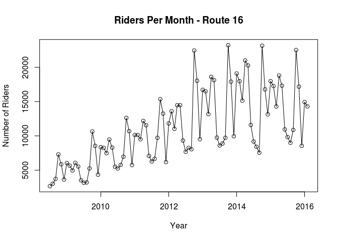
The time series plot suggest we can apply a seasonal model since there is a pattern. It also shows that there is an increasing trend over time, especially between years 2008-2013.
Model Specification
Data suggests an ARIMA(p,q,d) model. In order to reach stationarity, we look at possible transformations through a Box-Cox transformation with a 95% confidence interval and λ= 0.5.
Transformation
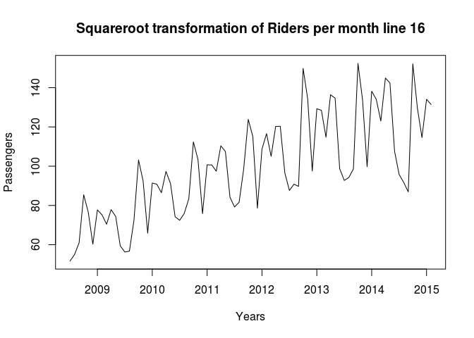
The output suggests a square root transformation.
1
2
3
4
5
  # Create subset of route 16 from Jan 2008 to Feb 2015
  route.16.window <- window(route.16, end=c(2015,2))

  # Use Box-Cox transformation to determine which power transf to use
  # BoxCox.ar(route.16.window)
Below is the plot of the transformed data:
1
  plot(sqrt(route.16.window),ylab="Passengers",xlab="Years",main="Squareroot transformation of Riders per month line 16")
Differentiation
The plot of the transformed data still shows stationarity, so we plot the first degree difference of the transformation. In addition to the stationarity, the plot still shows an increasing trend.
1
2
  # Differentiation
  plot(diff(sqrt(route.16.window),xlab="Years",ylab="First difference", main="First degree difference of the sqrt transformation"))
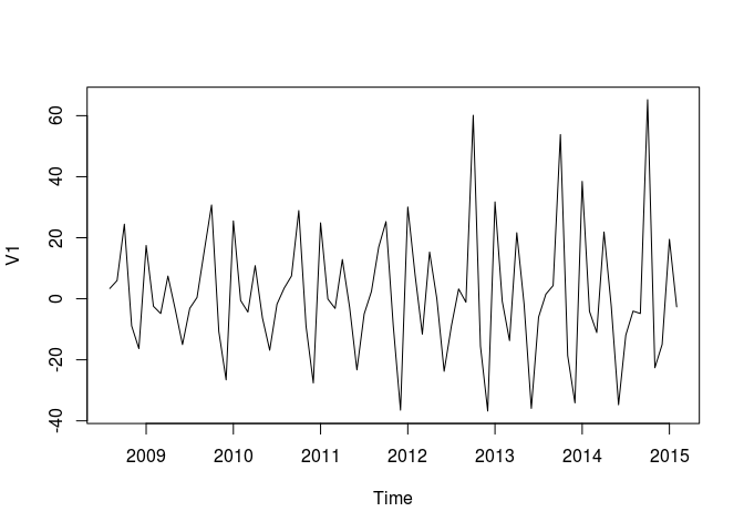
The Augmented Dickey-Fuller Test verifies the stationarity of the differentiated data with a p-value of 0.01. This value is sufficient to sustain the hypothesis that our data is stationary with a signficance level of α = 0.05.
1
2
3
4
5
6
7
8
9
  # Testing Stationarity
  adf.test(diff(sqrt(route.16.window)))

    ##
    ##  Augmented Dickey-Fuller Test
    ##
    ## data:  diff(sqrt(route.16.window))
    ## Dickey-Fuller = -6.8511, Lag order = 4, p-value = 0.01
    ## alternative hypothesis: stationary
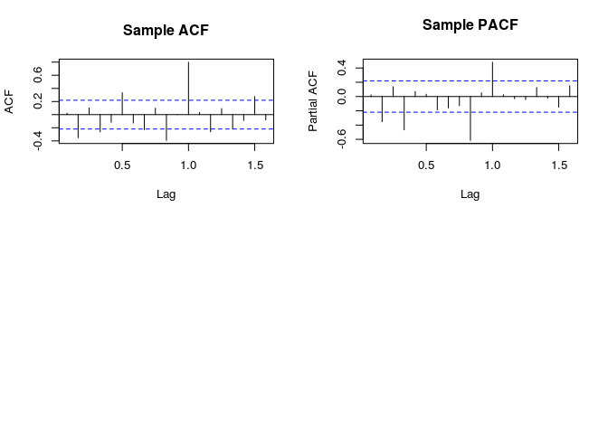
We can now proceed to find the appropriate ARMA(p,q) model by using the sample ACF and PACF with a lag of 12:
1
2
  # Sample ACF
  acf(as.vector(diff(sqrt(route.16.window),lag=12)))
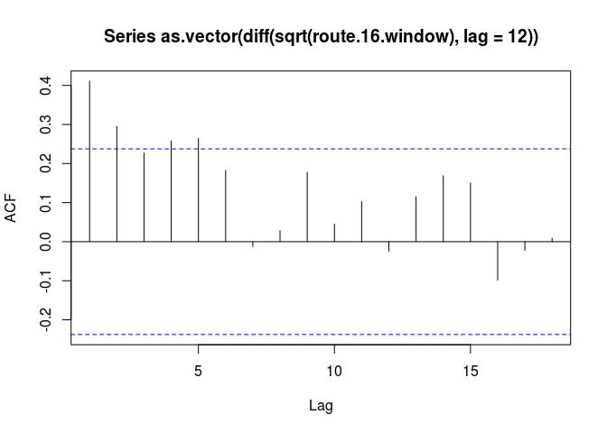
The Sample ACF resembles one of a seasonal MA(1) - it spikes at lag k = 1 and then drops below the margin of error. The Sample PACF also has a similar output.
1
2
  # Sample PACF
  pacf(as.vector(diff(sqrt(route.16.window),lag=12)))
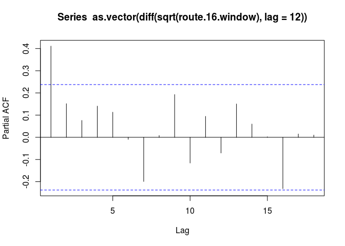
Both figures suggest that an ARIMA(1,1,1) model is most suitable for our data. To confirm this, we can also look at the EACF:
1
2
3
4
5
6
7
8
9
10
11
12
13
  # Sample EACF
  eacf(as.vector(diff(sqrt(route.16.window),lag=12)))

    ## AR/MA
    ##   0 1 2 3 4 5 6 7 8 9 10 11 12 13
    ## 0 x x o x x o o o o o o  o  o  o
    ## 1 x o o o o o o o o o o  o  o  o
    ## 2 x o o o o o o o o o o  o  o  o
    ## 3 x x x o o o o o x o o  o  o  o
    ## 4 x o o x o o o o o o o  o  o  o
    ## 5 x o o x o o o o o o o  o  o  o
    ## 6 o x o o o o o o o o o  o  o  o
    ## 7 o x o o x o o o o o o  o  o  o
The tip of the EACF is reached at the point (1,1), creating a wedge from there. In addition to the ARIMA(1,1,1) model, another suggested model for the data is an ARI(1,1) model since the sample ACF does not immediately drop below the margin of error. Different results can be obtained if the MA(1) of the ARIMA model is left out.
Model Fitting
Since we want to estimate how many people ride the bus each month, we will test two different approaches of our model, one with seasonality and one without it.
ARIMA(1,1,1) non-seasonal
1
2
3
4
5
6
7
8
9
10
11
12
13
14
  # ARIMA(1,1,1) non-seasonal
  arima111.ns.fit <- arima(sqrt(route.16.window), order=c(1,1,1), method='ML')
  arima111.ns.fit

    ##
    ## Call:
    ## arima(x = sqrt(route.16.window), order = c(1, 1, 1), method = "ML")
    ##
    ## Coefficients:
    ##          ar1      ma1
    ##       0.3046  -0.8660
    ## s.e.  0.1218   0.0487
    ##
    ## sigma^2 estimated as 315.9:  log likelihood = -339.87,  aic = 683.75
ARIMA(1,1,1) seasonal
1
2
3
4
5
6
7
8
9
10
11
12
13
14
15
  # ARIMA(1,1,1) seasonal
  arima111.fit <- arima(sqrt(route.16.window), order=c(1,1,1), seasonal=list(order=c(1,1,1), period=12), method="ML")
  arima111.fit

    ##
    ## Call:
    ## arima(x = sqrt(route.16.window), order = c(1, 1, 1), seasonal = list(order = c(1,
    ##     1, 1), period = 12), method = "ML")
    ##
    ## Coefficients:
    ##          ar1      ma1     sar1    sma1
    ##       0.2056  -0.8089  -0.8462  0.6708
    ## s.e.  0.1734   0.1168   0.3205  0.4487
    ##
    ## sigma^2 estimated as 36.52:  log likelihood = -217.05,  aic = 442.09
The following are the parameters:
which is equivalent to:
With ML estimates as \( \sigma^2_{e} \)≈ 315.9, \( \hat\phi \) = 0.3146, \( \hat\theta \) = -0.8660. The approximate 95% confidence intervals for \( \hat\phi \) and \( \hat\theta \) is (0.065872, 0.543328) and (-0.961452,-0.770548), respectively. We found that \( \hat\phi \) and \( \hat\theta \)are significantly different from 0.
ARI(1,1) non-seasonal
1
2
3
4
5
6
7
8
9
10
11
12
13
14
  # ARI(1,1) non-seasonal
  ari11.ns.fit <- arima(sqrt(route.16.window), order=c(1,1,0), method='ML')
  ari11.ns.fit

    ##
    ## Call:
    ## arima(x = sqrt(route.16.window), order = c(1, 1, 0), method = "ML")
    ##
    ## Coefficients:
    ##           ar1
    ##       -0.1733
    ## s.e.   0.1101
    ##
    ## sigma^2 estimated as 413.4:  log likelihood = -350.07,  aic = 702.15
ARI(1,1) seasonal
1
2
3
4
5
6
7
8
9
10
11
12
13
14
  ari11.fit <- arima(sqrt(route.16.window), order=c(1,1,0), seasonal=list(order=c(1,1,0), period=12), method="ML")
  ari11.fit

    ##
    ## Call:
    ## arima(x = sqrt(route.16.window), order = c(1, 1, 0), seasonal = list(order = c(1,
    ##     1, 0), period = 12), method = "ML")
    ##
    ## Coefficients:
    ##           ar1     sar1
    ##       -0.4081  -0.2667
    ## s.e.   0.1104   0.1282
    ##
    ## sigma^2 estimated as 44.52:  log likelihood = -222.77,  aic = 449.54
Model Diagnosis
Non-Seasonal Models
1
2
3
4
5
6
7
8
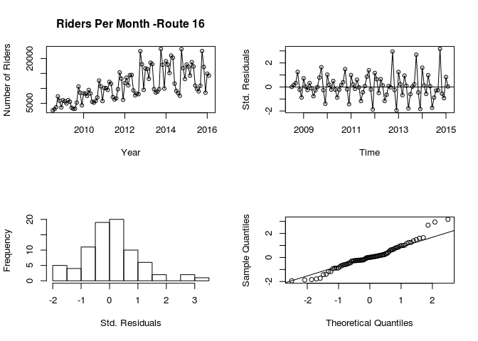
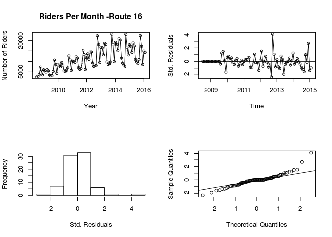
#ARI(1,1)
par(mfrow=c(2,2))
plot(route.16, ylab="Number of Riders", xlab="Year", main="Riders Per Month -Route 16",type="o")
plot(rstandard(ari11.ns.fit), ylab="Std. Residuals", xlab="Time", type="o")
abline(h=0)
hist(rstandard(ari11.ns.fit), xlab="Std. Residuals", main="")
qqnorm(rstandard(ari11.ns.fit), main="")
qqline(rstandard(ari11.ns.fit), main="")
Normality and Independence
1
2
3
4
5
6
7
8
9
10
11
12
13
14
15
16
17
18
19
20
21
22
23
24
25
26
27
28
29
30
31
32
33
34
35
36
37
38
39
40
41
42
43
44
45
46
47
48
49
50
51
52
53
54
55
56
57
58
  # Run Shapiro-Wilks test for normality
  shapiro.test(rstandard(ari11.ns.fit))

    ##
    ##  Shapiro-Wilk normality test
    ##
    ## data:  rstandard(ari11.ns.fit)
    ## W = 0.95787, p-value = 0.009997

  shapiro.test(rstandard(arima111.ns.fit))

    ##
    ##  Shapiro-Wilk normality test
    ##
    ## data:  rstandard(arima111.ns.fit)
    ## W = 0.97308, p-value = 0.08925

  # Runs test for Independence
  runs(rstandard(ari11.ns.fit))


    ## $pvalue
    ## [1] 0.916
    ##
    ## $observed.runs
    ## [1] 41
    ##
    ## $expected.runs
    ## [1] 40.975
    ##
    ## $n1
    ## [1] 39
    ##
    ## $n2
    ## [1] 41
    ##
    ## $k
    ## [1] 0

  runs(rstandard(arima111.ns.fit))

    ## $pvalue
    ## [1] 0.322
    ##
    ## $observed.runs
    ## [1] 35
    ##
    ## $expected.runs
    ## [1] 39.775
    ##
    ## $n1
    ## [1] 33
    ##
    ## $n2
    ## [1] 47
    ##
    ## $k
    ## [1] 0
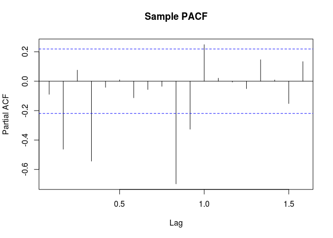
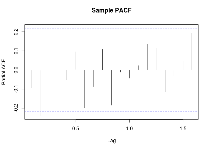
Residual PACF
1
2
  # Residual PACF
  pacf(rstandard(ari11.ns.fit), main="Sample PACF")
Overfitting
1
2
3
4
5
6
7
8
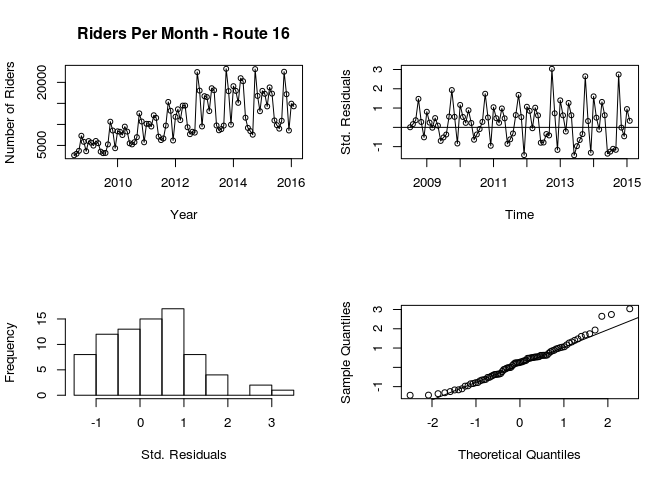
#ARIMA(1,1,1)
par(mfrow=c(2,2))
plot(route.16, ylab="Number of Riders", xlab="Year", main="Riders Per Month - Route 16",type="o")
plot(rstandard(arima111.ns.fit), ylab="Std. Residuals", xlab="Time", type="o")
abline(h=0)
hist(rstandard(arima111.ns.fit), xlab="Std. Residuals", main="")
qqnorm(rstandard(arima111.ns.fit), main="")
qqline(rstandard(arima111.ns.fit), main="")
1
2
3
4
  # Residual ACF / PACF
  par(mfrow=c(2,2))
  acf(rstandard(arima111.ns.fit), main="Sample ACF")
  pacf(rstandard(arima111.ns.fit), main="Sample PACF")
Seasonal Models
1
2
3
4
5
6
7
8
  #ARI(1,1)
  par(mfrow=c(2,2))
  plot(route.16, ylab="Number of Riders", xlab="Year", main="Riders Per Month -Route 16",type="o")
  plot(rstandard(ari11.fit), ylab="Std. Residuals", xlab="Time", type="o")
  abline(h=0)
  hist(rstandard(ari11.fit), xlab="Std. Residuals", main="")
  qqnorm(rstandard(ari11.fit), main="")
  qqline(rstandard(ari11.fit), main="")
Normality and Independence
1
2
3
4
5
6
7
8
9
10
11
12
13
14
15
16
17
18
19
20
21
22
23
24
25
26
27
28
29
30
31
32
33
34
35
36
37
38
39
40
41
42
43
44
45
46
47
48
49
50
51
52
53
54
55
56
57
  # Run Shapiro-Wilks test for normality
  shapiro.test(rstandard(ari11.fit))

    ##
    ##  Shapiro-Wilk normality test
    ##
    ## data:  rstandard(ari11.fit)
    ## W = 0.90862, p-value = 2.871e-05

  shapiro.test(rstandard(arima111.fit))

    ##
    ##  Shapiro-Wilk normality test
    ##
    ## data:  rstandard(arima111.fit)
    ## W = 0.91728, p-value = 7.093e-05

  # Runs test for Independence
  runs(rstandard(ari11.fit))

    ## $pvalue
    ## [1] 0.145
    ##
    ## $observed.runs
    ## [1] 34
    ##
    ## $expected.runs
    ## [1] 40.975
    ##
    ## $n1
    ## [1] 39
    ##
    ## $n2
    ## [1] 41
    ##
    ## $k
    ## [1] 0

  runs(rstandard(arima111.fit))

    ## $pvalue
    ## [1] 0.000994
    ##
    ## $observed.runs
    ## [1] 26
    ##
    ## $expected.runs
    ## [1] 40.975
    ##
    ## $n1
    ## [1] 41
    ##
    ## $n2
    ## [1] 39
    ##
    ## $k
    ## [1] 0
Residual PACF
1
2
  # Residual PACF
  pacf(rstandard(ari11.fit), main="Sample PACF")
Forecasting
To test our model, we withold observations from February 2015 to February 2016. The table below summarizes the actual values in March 2015 and January 2016 and the predictions estimated by the four ARIMA and ARI models.
| Time | Observation | ARIMA (1,1,1) Seasonal | ARI (1,1) Seasonal | ARIMA (1,1,1) Non-Seasonal | ARI (1,1) Non-Seasonal |
|---|---|---|---|---|---|
| March 2015 | 119.5 | 122.3 | 119.43 | 125.42 | 131.9 |
| January 2016 | 122.21 | 135.11 | 133.87 | 122.78 | 131.83 |